Dijkstra's Algorithm

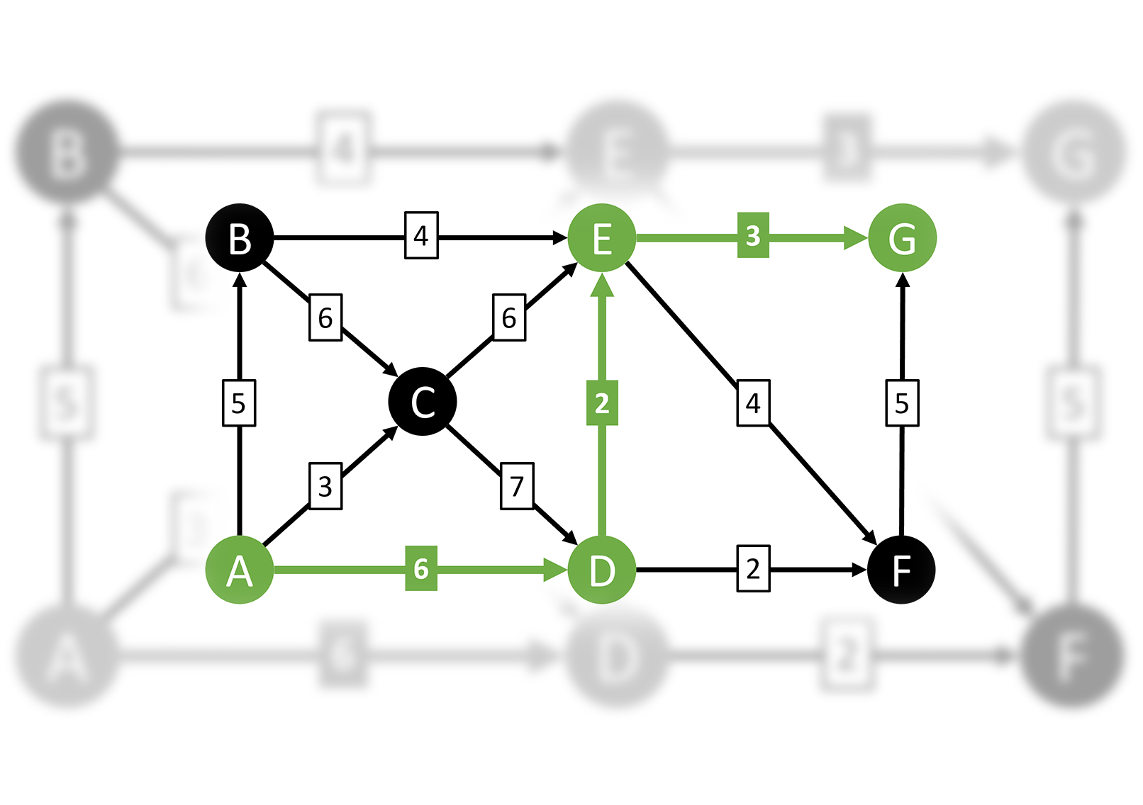
Dijkstra's SPF (shortest path first) algorithm calculates the shortest path from a starting node/vertex to all other nodes in a graph. This post describes how the algorithm works and how to implement it in Python as shown here: https://github.com/dmahugh/dijkstra-algorithm

The Wikipedia page for Dijkstra's algorithm has a good description of the basic concepts. Note that the distances between nodes must be positive or the algorithm may not work, and of course the starting node and destination node must be connected.

The algorithm creates a tree of the shortest distances from the starting node to all nodes in the graph, but in this example we're only concerned with finding the shortest path to the destination node. There are many variations and enhancements of Dijkstra's algorithm, such as the popular A* algorithm, which uses heuristics to determine which path to explore. In this post, we'll just focus on the original algorithm that Edsger Dijkstra came up with in 1959.

Finding the Shortest Path

Here's an example of a simple directed graph:

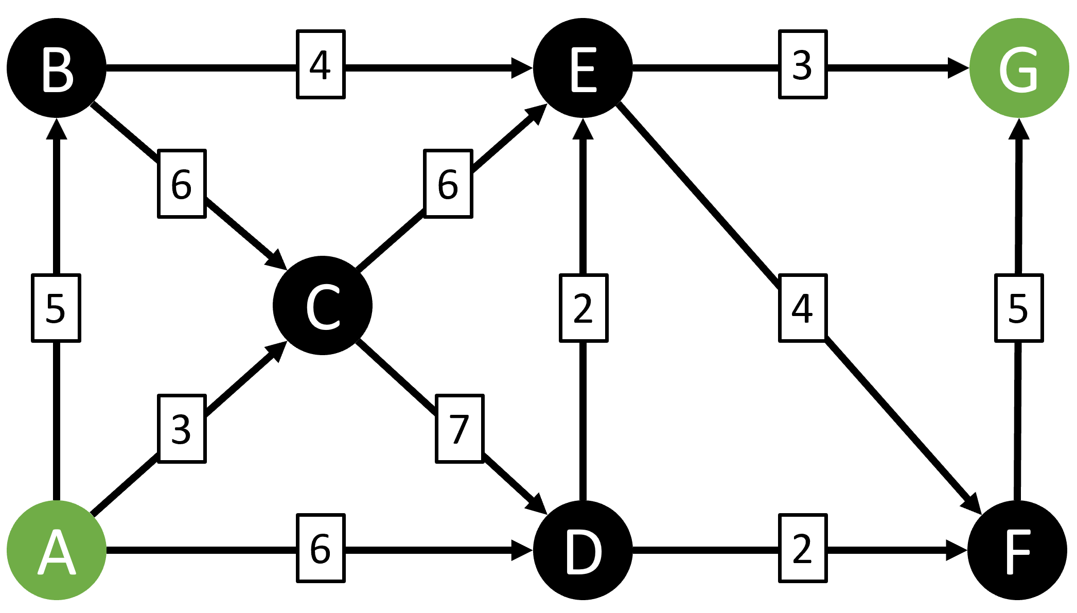
There are only 9 possible paths from A to G in this simple example, and you can manually work through them and quickly determine that the shortest path is A-D-E-G:

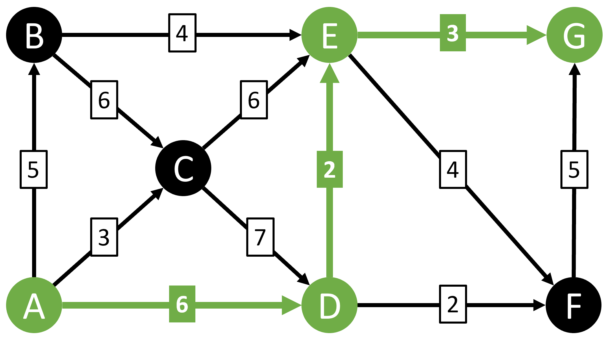
But what if we had a much larger graph with thousands of possible paths between two nodes? That's where Dijkstra's algorithm can help.

The Algorithm

Let's go through the steps in Dijkstra's algorithm (link) and see how they apply to the simple example above.

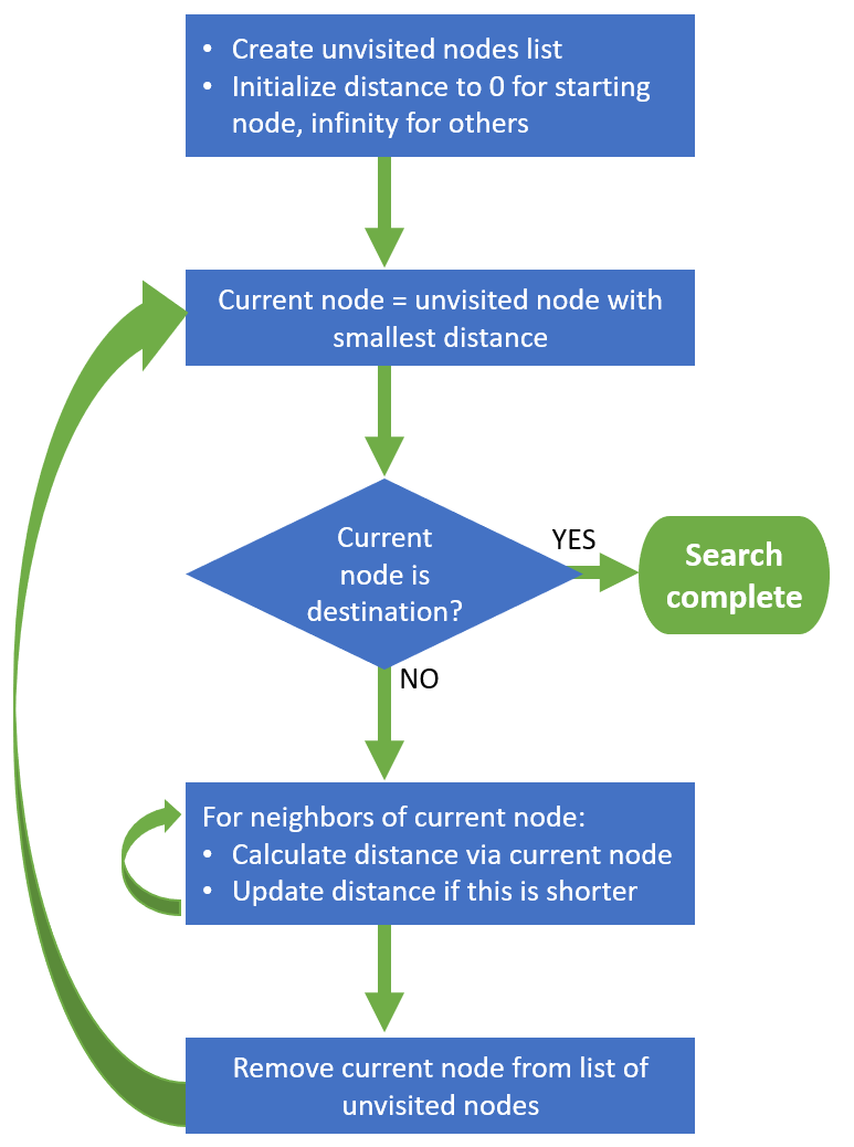
Step 1 is to create a list of the unvisited nodes. We haven't visited any nodes yet, so initially the unvisited list will contain all of the nodes in the graph: A, B, C, D, E, F, and G.

Step 2 is to create a table of the distance from the starting node to each of the nodes in the graph. The only distance we know at first is the distance from the starting node itself (A in our example), so we'll set that to 0. We'll then set the distance for all other nodes to infinity, and as we loop through the algorithm the central concept is that we'll be calculating new distances to the nodes along various paths and we replace a node's distance with a lower value whenever we find one.

Step 3 is the beginning of the main loop of the algorithm. We select as the current node the one that has the shortest distance stored for it. In our example, this will be A at first, which has a distance of 0.

Then we iterate through each of the neighbors of the current node (B, C, D in this example) and calculate the distance from the starting node to this neighbor node on the path through our "current node." In other words, we add the current node's stored distance (0 in our example) to the distance from the current node to the neighbor (in our example, B=5, C=3, D=6). We compare the new calculated distance to the distance we already have for each neighbor, and update the distance to the minimum of these two values. In our first loop for the example graph, B/C/D all have infinity for their stored distance, so the calculated distance of 5/3/6 is lower and will be stored as the distance for B/C/D.

Step 4 is to simply remove the visited node (A in this example) from the unvisited list.

Step 5 is to check whether we're done, and if so break out of the main loop. There are three possible conditions that can terminate the algorithm:

• We've visited all of the nodes.
• We've visited the destination node.
• The shortest distance for any of the remaining unvisited nodes is infinity. (This will happen if there are nodes that are not connected in any way to the starting node.)

Step 6 is to loop back to Step 3. In our example, C will be the current node on the next pass through the loop, because it now has the shortest stored distance (3).

Now let's look at how to implement this in code.

Python Implementation

You can find a complete implementation of the Dijkstra algorithm in dijkstra_algorithm.py.

All the heavy lifting is done by the Graph class, which gets initialized with a graph definition and then provides a shortest_path method that uses the Dijkstra algorithm to calculate the shortest path between any two nodes in the graph. There is also a main function that includes a few simple test cases to verify the algorithm.

The graph definition is stored in a text file, with each line specifying an edge of the graph in this format: start_node<space>end_node<space>distance. The Graph constructor reads that file and builds two data structures as properties: a set of nodes, and a dictionary containing the adjacency list for each node.

The heart of the algorithm (described in Step 3 earlier) is when we iterate through the current node's neighbors and calculate the total distance to each neighbor from the start node via the current node. Here's how that is implemented in the shortest_path method:

# For each neighbor of current_node, check whether the total distance
# to the neighbor via current_node is shorter than the distance we
# currently have for that node. If it is, update the neighbor's values
# for distance_from_start and previous_node.
for neighbor, distance in self.adjacency_list[current_node]:
    new_path = distance_from_start[current_node] + distance
    if new_path < distance_from_start[neighbor]:
        distance_from_start[neighbor] = new_path
        previous_node[neighbor] = current_node

When the algorithm terminates, we return both the path and the total distance. We already know the distance for each visited node, so we can just look it up in the distance_from_start dictionary, but the path needs to be built as shown here from the previous_node dictionary.

The sample repo contains two graph definition files: simple_graph.txt, which defines the graph we used in the example above, and seattle_area.txt, which defines a graph of a few locations around the Seattle area:

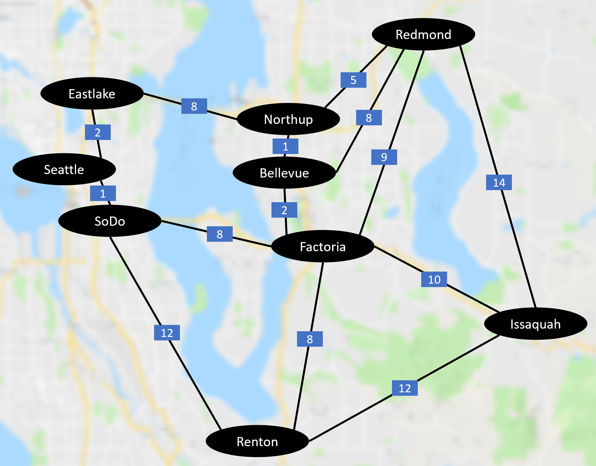
Note that the seattle_area.txt graph definition includes every edge defined in both directions, which essentially makes it an undirected graph.

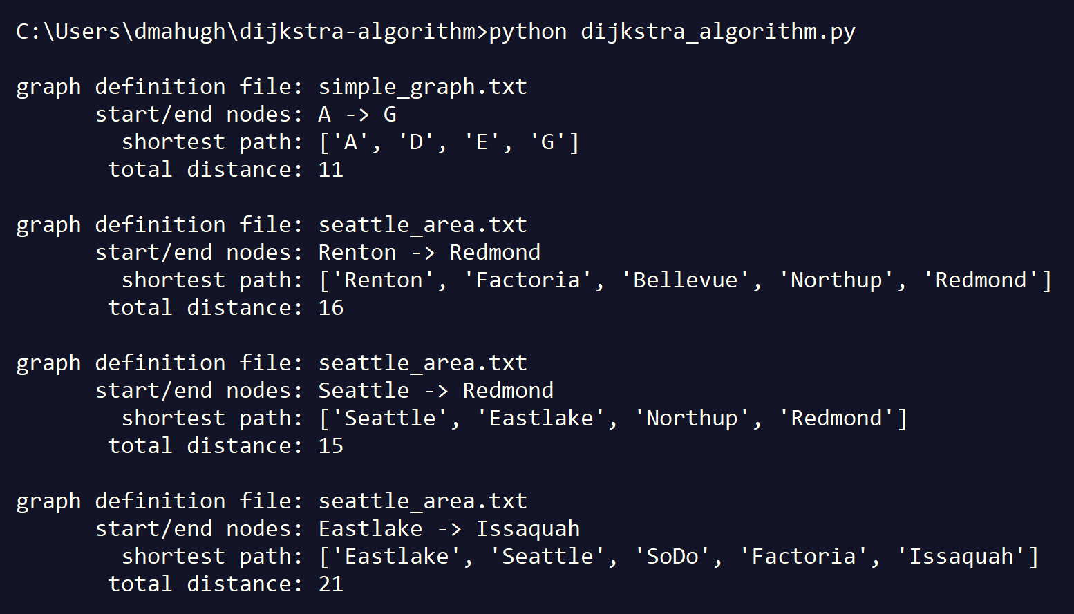
Here's an example of the output of the sample:

I hope this example helps you understand the Dijkstra algorithm!